
Last Updated June 28, 2026
Satellite crop monitoring for crop forecasting and area assessment works best when every image answers a defined crop question: what is planted, how much area it covers, how the canopy is changing, and whether the season is moving toward a realistic yield range. A green field on a screen is the beginning. The value appears when field boundaries, crop labels, weather, ground checks, and yield records turn the image into a measurement that can survive a muddy boots check.
Good satellite work feels like reading a field notebook from above. The same corn field can look dark green after a rain, pale after hail, striped from planter skips, or patchy from drowned-out low spots. Crop forecasts become useful when those visual signals are separated from acreage, crop type, soil moisture, planting date, and the growth stage that made the signal appear.
Key Takeaways
- Separate crop area, crop condition, and yield forecasting.
- Use ground checks before trusting acreage or stress maps.
- Match sensor choice to clouds, field size, and crop stage.
- Avoid forecasting from one image date or one index.
- Review errors after harvest and update field labels.
Table of Contents
Satellite Crop Monitoring Starts With A Clear Forecasting Target
Satellite imagery can support crop forecasting, acreage estimation, disaster assessment, irrigation planning, and early warning. Accuracy drops when all of those jobs are blended into one map. A forecast model needs a different kind of confidence than a planted-area estimate, and a drought alert needs a different time window than a harvest forecast.
Crop monitoring becomes more reliable when three layers stay separate. Area assessment identifies the crop and measures the planted or harvested area. Condition monitoring tracks canopy change, soil moisture, heat stress, flood damage, or delayed growth. Production forecasting combines area and expected yield with weather, crop stage, field history, and ground checks.
The separation matters in the field. Accurate crop area can still miss yield after pollination heat. Dense canopy on an NDVI map can hide disease in the lower leaves. Dryland wheat may look weak in April and recover after a cool, wet May. The satellite signal is a clue, and the forecast comes from how that clue is tied to crop biology and timing.
| Forecast Question | Satellite Signal | Needed Ground Data | Decision It Supports |
|---|---|---|---|
| What crop is growing? | Seasonal reflectance pattern and crop classification | Field labels, planting records, known rotations | Crop inventory and acreage reporting |
| How much area is planted? | Field boundary plus crop map | Boundary edits, prevented planting notes, double-crop checks | Area assessment and supply estimates |
| Is the stand developing normally? | Early canopy cover and emergence pattern | Planting date, stand counts, replant records | Replant review and early yield risk |
| Where is the crop under stress? | Vegetation index, moisture, thermal, or radar anomaly | Scouting notes, soil moisture, rainfall, pest pressure | Scouting priority and treatment timing |
| What yield range is likely? | Time-series canopy and weather-linked growth signal | Yield history, crop stage, harvest data, local management | Storage, marketing, labor, and logistics planning |
Machine learning yield forecasting becomes stronger when satellite signals are treated as measured inputs in a larger crop model. A model still needs crop stage, weather timing, field history, and validation against harvested yield.
Crop Area Assessment Separates Crop Type, Field Boundary, And Acreage
Area assessment sounds simple until the map meets real fields. Crop type, field boundary, planted area, harvested area, and prevented planting can all differ. A clean rectangle on a satellite image may include waterways, tree shadows, a farm lane, drowned-out corners, or a cover crop strip that confuses classification.
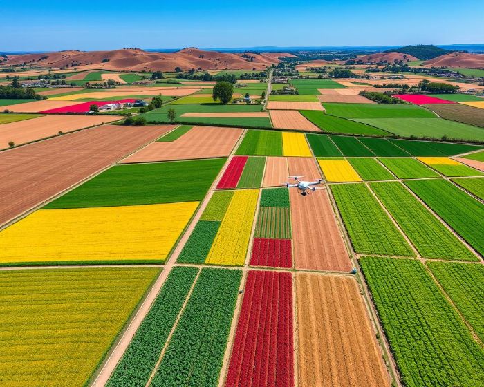
Crop classification uses a season of images across planting, canopy closure, maturity, and harvest. Corn, soybeans, wheat, rice, cotton, and alfalfa each change color, density, texture, and timing in different ways. Winter wheat greens early, corn closes rows later, and double-crop soybeans can appear after small-grain harvest. The time pattern carries more value than one bright green image.
For U.S. acreage work, public cropland tools already support crop acreage assessment and crop-specific land cover change detection. The 2025 Cropland Data Layer announcement also reports a 10-meter spatial resolution beginning with 2024 data, which helps reduce mixed-pixel problems in smaller fields, field edges, and narrow crop blocks.
Boundary quality can be the quiet source of big errors. If a field polygon includes a grassy drainage swale, the crop area is inflated. If a headland is cut off, yield per acre can look too high after harvest. Boundary edits should happen before the crop model is judged, because a sharp model built on a sloppy field outline still produces a sloppy estimate.
Pro Tip: Check three boundary spots before accepting an area estimate: the field entrance, the lowest wet corner, and the edge beside trees or buildings. Those places often create the first acreage and crop-type errors.
Vegetation Indices Turn Canopy Reflectance Into Crop Condition Signals
Healthy leaves absorb visible red light for photosynthesis and reflect near-infrared light from their internal structure. Vegetation indices such as NDVI use that difference to show where a canopy is dense, thin, delayed, or damaged. The result can be a useful crop condition signal, especially when the same field is compared across dates.
NDVI has limits. It can saturate in dense corn or soybean canopy, which means very good and excellent growth can look similar. It can also respond to weeds, cover crops, or wet soil near the crop row. A map that looks smooth from a desk may feel very different when leaves are curled, mud sticks to boots, and the low ground smells sour after water sits too long.
Other indices and sensors add texture. Red-edge bands can catch canopy changes before a visible color shift is obvious. Thermal data can show heat and water stress. Radar can help when clouds block optical imagery, and soil moisture products can show where a rain event never reached the root zone. Each layer needs timing context. A pale field after emergence means something different from a pale field after pollination.
Common Satellite Crop Monitoring Indices And What They Show
| Index Or Signal | What It Reads | Best Use | Main Caution |
|---|---|---|---|
| NDVI | Red and near-infrared canopy contrast | General crop vigor, emergence, canopy trend, and stress screening | Saturates in dense canopy and can respond to weeds or wet soil |
| EVI or EVI2 | Canopy vigor with reduced soil and atmospheric noise | Dense crop canopies where NDVI becomes less responsive | Still needs crop-stage timing and clean image correction |
| Red-edge chlorophyll indices | Subtle canopy and chlorophyll shifts | Nitrogen stress, early canopy change, and crop condition comparison | Needs sensor bands that include red-edge wavelengths |
| NDWI or NDMI | Water-related canopy or moisture response | Drought screening, irrigation review, and water-stress comparison | Can be confused by soil, residue, crop stage, and recent rain |
| VCI or VHI | Vegetation condition compared with history, often with thermal stress | Drought monitoring, regional crop condition, and production-risk alerts | Less useful for rapid field diagnosis when the signal is lagged or coarse |
| Thermal anomaly | Canopy temperature and heat stress | Irrigation timing, drought stress, and crop-water review | Needs weather context and time-of-day control |
| Radar backscatter | Canopy structure and surface moisture response | Cloudy regions, flood assessment, and weather-gap filling | Needs local calibration |
Predictive analytics for crop health can use satellite anomalies as scouting triggers when disease, nutrient stress, insects, or water problems create similar canopy patterns. The map should narrow the walking route, then field checks should identify the cause.
A condition map earns trust when the same pattern still makes sense after walking the headlands, opening the canopy with both hands, and checking the roots, leaves, and soil surface.

Forecast Accuracy Improves When Satellite Data Is Joined To Ground Truth
Ground truth is the correction layer that keeps satellite forecasting honest. It includes field labels, crop stage notes, planting dates, stand counts, soil moisture readings, scouting notes, yield monitor data, weigh tickets, and local weather. A missing ground layer can make a forecast confuse late planting with poor crop vigor or clean fallow soil with crop failure.
Strong crop forecasts usually use time series. One image can be cloudy, smoky, shadowed, or taken during a short stress pulse. A sequence shows whether the canopy recovered, declined, stalled, or advanced normally. The texture of the trend matters: a slow climb after delayed planting has a different risk profile than a sharp drop after flooding.
Operational crop-monitoring systems use satellite data to provide timely insights on crop conditions for early warning and planning. That operational use is a good reminder that satellite forecasting works at several scales. A national wheat outlook may tolerate county-level uncertainty. A farm input decision often needs field-level confidence.
Field sensors can improve the same pipeline when they measure the stress factor the image cannot explain. Garden and farm IoT devices earn their place when soil moisture, temperature, leaf wetness, or station data are maintained through the season and tied to exact field zones. A sensor sitting in the wrong soil type can mislead the satellite model with very tidy numbers.
Field Note: Weak forecasts often share one habit: they trust the cleanest-looking map date and ignore the field note that explains why that date was unusual.
Choose The Right Satellite Data Source By Scale And Weather Risk
The best data source depends on the crop question, the field size, the weather pattern, and how quickly a decision must be made. Free public imagery may be enough for regional acreage and weekly condition tracking. High-resolution commercial imagery may be needed for small fields, specialty crops, narrow beds, or within-field management zones.
Clouds are the classic problem for optical imagery. A cloudy week during emergence, flowering, flood recovery, or drought stress can remove the most valuable date from the record. Radar helps in cloudy regions because it can collect through clouds and respond to canopy structure and surface moisture. It also takes more skill to interpret, especially where rough soil, residue, and crop height change together.
Sentinel-2 is often the practical starting point for satellite crop monitoring because its multispectral bands support vegetation, moisture, and canopy-change analysis at field-relevant resolution. The mission provides 13 spectral bands across 10 m, 20 m, and 60 m resolutions, so the useful layer depends on the crop question, field size, cloud cover, and growth stage.
| Data Layer | Best Signal | Strength | Weak Point |
|---|---|---|---|
| Optical imagery | Leaf color, canopy density, vegetation indices | Easy to interpret and strong for crop condition | Blocked by clouds, smoke, and shadows |
| Radar imagery | Canopy structure and surface moisture response | Works through clouds and can fill weather gaps | Needs local calibration |
| Thermal imagery | Canopy heat and water stress | Useful for drought, irrigation, and heat stress | Needs careful timing and weather context |
| High-resolution imagery | Field edges, small blocks, stand gaps | Better for specialty crops and small fields | Higher cost and uneven revisit timing |
| Weather and soil moisture data | Rainfall, heat, evapotranspiration, root-zone water | Explains why the canopy changed | Can be coarse when local sensors are absent |
Irrigation data analytics becomes more useful when satellite canopy stress is joined with root-zone moisture, rainfall, evapotranspiration, and crop stage. A hot canopy calls for a different response when the root zone is dry than when disease or compaction is restricting uptake.
Turn Satellite Crop Forecasts Into Farm And Policy Decisions
A forecast earns attention when it changes a decision. At the farm level, satellite data can guide scouting, irrigation checks, variable-rate priorities, replant discussions, harvest sequencing, and storage planning. At regional scale, it can support acreage estimates, crop condition reports, food security monitoring, disaster response, and market transparency.
Early warning work depends on timing. Crop stress that appears after the main yield window may explain a loss, with little time left to prevent much of it. Stress detected before flowering, grain fill, tuber bulking, or fruit sizing can still shape irrigation, fertility, pest scouting, and logistics. The right forecast tells a manager which action still has time to matter.
Global crop monitoring networks use satellite monitoring for early warning of production shortfalls. That scale is different from field management, and the same logic applies: crop type, area, condition, weather, and ground reports have to line up before the forecast should influence supply, aid, or purchasing decisions.
Automated systems can act on satellite-derived zones when the prescription is tied to equipment limits, product labels, and crop stage. Automated crop management works best when the map class leads to a specific action, such as scouting, irrigation review, or variable-rate adjustment.
Common Failure Modes In Satellite Crop Forecasting
Satellite forecasts usually fail in ordinary ways. The image date is wrong for the crop stage. The field boundary includes non-crop ground. A stress map detects symptoms and leaves the cause unknown. The model trained in one region is moved to another region with different soils, hybrids, planting dates, or irrigation practices.
The best correction is a short error review after harvest. Compare the forecast with actual yield, mark the fields where the model missed badly, and write down the cause before the season fades from memory. Hail, replanting, flood damage, late nitrogen, herbicide injury, plugged emitters, and harvest loss each leave a different story behind the same low-yield pixel.
| Problem | Visible Sign | Why It Misleads | Correction |
|---|---|---|---|
| Cloud or shadow gaps | Missing or dark patches on key dates | Stress or recovery is hidden during the decision window | Use radar, later dates, and field notes |
| Mixed pixels | Edges look like crop, grass, road, and trees together | Acreage and condition estimates drift near boundaries | Edit boundaries and remove non-crop strips |
| Crop confusion | Similar growth curves in nearby crops | Area assessment assigns the wrong crop class | Add field labels and rotation history |
| Late planting or replanting | Field looks weak compared with neighbors | The model reads timing delay as yield damage | Add planting and replant dates |
| Sparse ground truth | Map looks precise, field checks are few | Local causes are inferred from canopy color alone | Scout representative high, medium, and low zones |
| Region transfer | Good results in one county, poor results elsewhere | Soils, varieties, rainfall, and management changed | Validate by region before using the forecast |
A forecast should carry a confidence note when weather gaps, missing labels, or weak validation affect the result. That note is more useful than a false decimal. A yield range of 165 to 178 bushels per acre with clear assumptions can guide planning better than a single 172.4 number that hides uncertainty.
Conclusion
Satellite data improves crop forecasting when it is used as a disciplined measurement system: crop type first, acreage second, condition trend third, yield forecast only after the ground evidence is attached. If the field boundary is wrong or the growth stage is missing, even a sharp image can send the forecast in the wrong direction.
After each season, compare the forecast with harvested yield, mark the fields where error exceeded a useful threshold, and record the reason within two weeks of harvest. The best system leaves behind cleaner field labels, better timing notes, and maps that match what a person saw walking the rows.
FAQ
How accurate is satellite data for crop forecasting?
Accuracy depends on crop type, field size, image timing, ground truth, weather gaps, and the forecast scale. Regional forecasts can work with coarser data. Field-level yield estimates need clean boundaries, crop-stage timing, and harvest validation.
Can satellite imagery estimate crop acreage?
Yes, satellite imagery can estimate crop acreage when crop classification is joined with reliable field boundaries and crop labels. The estimate should be checked for roads, waterways, tree shadows, prevented planting, double cropping, and mixed pixels along edges.
Which satellite index is most used for crop monitoring?
NDVI is the most familiar vegetation index for crop monitoring because it uses red and near-infrared reflectance to track green canopy strength. Dense canopy, weeds, wet soil, and crop stage can distort the signal, so time-series comparison is safer than one-date interpretation.
Do satellites replace field scouting?
Satellites make field scouting more targeted. A map can show where the canopy changed, then scouting identifies whether the cause is drought, insects, disease, nutrient stress, compaction, flooding, or management history.